#install.packages("usethis")
usethis::use_course("https://github.com/r-journalism/nicar-2024-tidycenus/archive/master.zip")

# Run this in the console of RStudio
file.edit("02_wrangling_census_data.R")Wrangling (Census) data
You can follow along with the 02_wrangling_census_data file in the nicar-2024-tidycensus-viz project folder that you downloaded in the intro link.
The repo containing the data and scripts for this section is on Github. To install those files, run the lines of code below.
To follow along with this walkthrough, simply run the lines of code in the gray boxes in the R console. Be sure to run them in order. If you run into an error, it may be because you skipped running some preceding lines of code.
Tidycensus functions
The basics to wrangle data
filter()gets rid of rowsmutate()adds columns to the dataframegroup_by()andsummarize()will aggregate the data by groupsarrange()will sort the dataselect()will help narrow down columns- Daisy chain all these functions together with
|>
Case study: Racial plurality by county
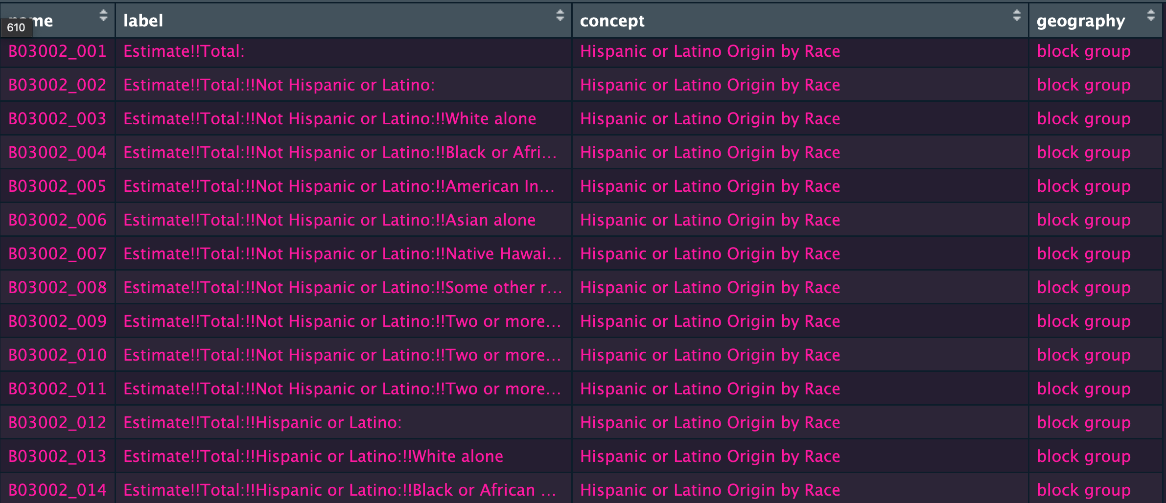
View(vars) # and search for Hispanic or Latino Origin by RaceLoad libraries
library(tidyverse)
library(tidycensus)
Download race Census data
county_diversity <- get_acs(geography = "county",
                            variables = c("B03002_001", # total
                                          "B03002_003", # white alone
                                          "B03002_004", # black alone
                                          "B03002_005", # native american
                                          "B03002_006", # asian alone
                                          "B03002_007", # pi alone
                                          "B03002_012" # hispanic or latino
                            ),
                            survey="acs5",
                            year=2022)
Getting data from the 2018-2022 5-year ACScounty_diversity# A tibble: 22,554 × 5
GEOID NAME variable estimate moe
<chr> <chr> <chr> <dbl> <dbl>
1 01001 Autauga County, Alabama B03002_001 58761 NA
2 01001 Autauga County, Alabama B03002_003 42635 224
3 01001 Autauga County, Alabama B03002_004 11496 525
4 01001 Autauga County, Alabama B03002_005 59 71
5 01001 Autauga County, Alabama B03002_006 636 213
6 01001 Autauga County, Alabama B03002_007 0 30
7 01001 Autauga County, Alabama B03002_012 1864 NA
8 01003 Baldwin County, Alabama B03002_001 233420 NA
9 01003 Baldwin County, Alabama B03002_003 192161 1020
10 01003 Baldwin County, Alabama B03002_004 19318 730
# ℹ 22,544 more rowsAdd a total population column
- With an argument
summary_var
county_diversity <- get_acs(geography = "county",
                            variables = c("B03002_003", # white alone
                                          "B03002_004", # black alone
                                          "B03002_005", # native american
                                          "B03002_006", # asian alone
                                          "B03002_007", # pi alone
                                          "B03002_012" # hispanic or latino
                            ),
                            summary_var = "B03002_001", # total population
                            survey="acs5",
                            year=2022)
Getting data from the 2018-2022 5-year ACScounty_diversity# A tibble: 19,332 × 7
GEOID NAME variable estimate moe summary_est summary_moe
<chr> <chr> <chr> <dbl> <dbl> <dbl> <dbl>
1 01001 Autauga County, Alabama B03002_… 42635 224 58761 NA
2 01001 Autauga County, Alabama B03002_… 11496 525 58761 NA
3 01001 Autauga County, Alabama B03002_… 59 71 58761 NA
4 01001 Autauga County, Alabama B03002_… 636 213 58761 NA
5 01001 Autauga County, Alabama B03002_… 0 30 58761 NA
6 01001 Autauga County, Alabama B03002_… 1864 NA 58761 NA
7 01003 Baldwin County, Alabama B03002_… 192161 1020 233420 NA
8 01003 Baldwin County, Alabama B03002_… 19318 730 233420 NA
9 01003 Baldwin County, Alabama B03002_… 512 187 233420 NA
10 01003 Baldwin County, Alabama B03002_… 2046 347 233420 NA
# ℹ 19,322 more rowsAdd a percent column
- Using the dplyr library of data wrangling functions
mutate()to add a new column to the data frame
library(dplyr)

county_diversity <- county_diversity |>
mutate(percent=estimate/summary_est*100)county_diversity# A tibble: 19,332 × 7
GEOID NAME variable estimate moe summary_est percent
<chr> <chr> <chr> <dbl> <dbl> <dbl> <dbl>
1 01001 Autauga County, Alabama B03002_003 42635 224 58761 72.6
2 01001 Autauga County, Alabama B03002_004 11496 525 58761 19.6
3 01001 Autauga County, Alabama B03002_005 59 71 58761 0.100
4 01001 Autauga County, Alabama B03002_006 636 213 58761 1.08
5 01001 Autauga County, Alabama B03002_007 0 30 58761 0
6 01001 Autauga County, Alabama B03002_012 1864 NA 58761 3.17
7 01003 Baldwin County, Alabama B03002_003 192161 1020 233420 82.3
8 01003 Baldwin County, Alabama B03002_004 19318 730 233420 8.28
9 01003 Baldwin County, Alabama B03002_005 512 187 233420 0.219
10 01003 Baldwin County, Alabama B03002_006 2046 347 233420 0.877
# ℹ 19,322 more rowsAdd better variable names
case_when()to refactor values (withinmutate()).defaultis else or if none of the factors match|>are the new pipes, aka “and then”
county_diversity_race <- county_diversity |>
  mutate(race=case_when(
    variable=="B03002_003" ~"White",
    variable=="B03002_004" ~"Black",
    variable=="B03002_005" ~"Native American",
    variable=="B03002_006" ~"Asian",
    variable=="B03002_007" ~"Pacific Islander",
    variable=="B03002_012" ~"Hispanic",
    .default = "Other"
))county_diversity_race# A tibble: 19,332 × 6
GEOID NAME estimate summary_est percent race
<chr> <chr> <dbl> <dbl> <dbl> <chr>
1 01001 Autauga County, Alabama 42635 58761 72.6 White
2 01001 Autauga County, Alabama 11496 58761 19.6 Black
3 01001 Autauga County, Alabama 59 58761 0.100 Native American
4 01001 Autauga County, Alabama 636 58761 1.08 Asian
5 01001 Autauga County, Alabama 0 58761 0 Pacific Islander
6 01001 Autauga County, Alabama 1864 58761 3.17 Hispanic
7 01003 Baldwin County, Alabama 192161 233420 82.3 White
8 01003 Baldwin County, Alabama 19318 233420 8.28 Black
9 01003 Baldwin County, Alabama 512 233420 0.219 Native American
10 01003 Baldwin County, Alabama 2046 233420 0.877 Asian
# ℹ 19,322 more rowsGroup up some smaller groups
- use
group_by()to group up things - use
summarize()to do something (usually math) on these groups - Let’s combine the population for Asian and Pacific Islander
Group up some smaller groups code
county_diversity_percent <- county_diversity |>
  mutate(race=case_when(
    variable=="B03002_003" ~"White",
    variable=="B03002_004" ~"Black",
    variable=="B03002_005" ~"Native American",
    variable=="B03002_006" ~"Asian Pacific Islander",
    variable=="B03002_007" ~"Asian Pacific Islander",
    variable=="B03002_012" ~"Hispanic",
    .default = "Other"
  )) |>
  group_by(GEOID, NAME, race) |>
  summarize(estimate=sum(estimate, na.rm=T),
            summary_est=mean(summary_est, na.rm=T)) |>
  mutate(percent=estimate/summary_est*100)
`summarise()` has grouped output by 'GEOID', 'NAME'. You can override using the
`.groups` argument.county_diversity_percent# A tibble: 16,110 × 5
NAME race estimate summary_est percent
<chr> <chr> <dbl> <dbl> <dbl>
1 Autauga County, Alabama Asian Pacific Islander 636 58761 1.08
2 Autauga County, Alabama Black 11496 58761 19.6
3 Autauga County, Alabama Hispanic 1864 58761 3.17
4 Autauga County, Alabama Native American 59 58761 0.100
5 Autauga County, Alabama White 42635 58761 72.6
6 Baldwin County, Alabama Asian Pacific Islander 2068 233420 0.886
7 Baldwin County, Alabama Black 19318 233420 8.28
8 Baldwin County, Alabama Hispanic 11210 233420 4.80
9 Baldwin County, Alabama Native American 512 233420 0.219
10 Baldwin County, Alabama White 192161 233420 82.3
# ℹ 16,100 more rowsSort the data frame low to high
- Use the
arrange()function
county_diversity_percent |>
  group_by(NAME) |>
  arrange(NAME, percent)
# A tibble: 16,110 × 4
NAME race estimate percent
<chr> <chr> <dbl> <dbl>
1 Abbeville County, South Carolina Native American 28 0.115
2 Abbeville County, South Carolina Asian Pacific Islander 58 0.238
3 Abbeville County, South Carolina Hispanic 441 1.81
4 Abbeville County, South Carolina Black 6372 26.1
5 Abbeville County, South Carolina White 16658 68.4
6 Acadia Parish, Louisiana Native American 13 0.0225
7 Acadia Parish, Louisiana Asian Pacific Islander 95 0.165
8 Acadia Parish, Louisiana Hispanic 1780 3.09
9 Acadia Parish, Louisiana Black 9511 16.5
10 Acadia Parish, Louisiana White 44413 77.0
# ℹ 16,100 more rowsSort the data frame high to low
- Use the
arrange()function - Use the
desc()function
county_diversity_percent_sorted <- county_diversity_percent |>
  group_by(NAME) |>
arrange(NAME, desc(percent))county_diversity_percent_sorted# A tibble: 16,110 × 5
NAME race estimate summary_est percent
<chr> <chr> <dbl> <dbl> <dbl>
1 Abbeville County, South Carolina White 16658 24368 68.4
2 Abbeville County, South Carolina Black 6372 24368 26.1
3 Abbeville County, South Carolina Hispanic 441 24368 1.81
4 Abbeville County, South Carolina Asian Pacific … 58 24368 0.238
5 Abbeville County, South Carolina Native American 28 24368 0.115
6 Acadia Parish, Louisiana White 44413 57674 77.0
7 Acadia Parish, Louisiana Black 9511 57674 16.5
8 Acadia Parish, Louisiana Hispanic 1780 57674 3.09
9 Acadia Parish, Louisiana Asian Pacific … 95 57674 0.165
10 Acadia Parish, Louisiana Native American 13 57674 0.0225
# ℹ 16,100 more rowsNotice there are 16,110 rows…
Narrow down the rows
- We want one row for every county
- Use the
filter()function
county_diversity_percent_plurality <-
  county_diversity_percent |>
  group_by(NAME) |>
  arrange(NAME, desc(percent)) |>
filter(row_number()==1)county_diversity_percent_plurality# A tibble: 3,222 × 5
NAME race estimate summary_est percent
<chr> <chr> <dbl> <dbl> <dbl>
1 Abbeville County, South Carolina White 16658 24368 68.4
2 Acadia Parish, Louisiana White 44413 57674 77.0
3 Accomack County, Virginia White 19813 33367 59.4
4 Ada County, Idaho White 411348 497494 82.7
5 Adair County, Iowa White 7046 7479 94.2
6 Adair County, Kentucky White 17308 18887 91.6
7 Adair County, Missouri White 22367 25299 88.4
8 Adair County, Oklahoma Native American 8468 19726 42.9
9 Adams County, Colorado White 247045 520149 47.5
10 Adams County, Idaho White 4009 4464 89.8
# ℹ 3,212 more rowsNow there are 3,222 rows.
Which lines up with the county count in the U.S.
Narrow down the rows II
- Use the
slice()function
county_diversity_percent_plurality <-
  county_diversity_percent |>
  group_by(NAME) |>
  arrange(NAME, desc(percent)) |>
  slice(1)
Case study: Evictions in San Diego
sd_evictions <- read_csv("san_diego_evictions.csv")Rows: 736 Columns: 2
── Column specification ────────────────────────────────────────────────────────
Delimiter: ","
chr (1): GEOID
dbl (1): total_evictions
ℹ Use `spec()` to retrieve the full column specification for this data.
ℹ Specify the column types or set `show_col_types = FALSE` to quiet this message.sd_evictions# A tibble: 736 × 2
GEOID total_evictions
<chr> <dbl>
1 06073000100 1
2 06073000201 2
3 06073000202 4
4 06073000301 2
5 06073000302 10
6 06073000400 6
7 06073000500 3
8 06073000600 2
9 06073000700 3
10 06073000800 20
# ℹ 726 more rowsGo back and modify your code
Copy and paste over the code you worked so hard on and change the geography and add state and county.
sd_tract_diversity <- get_acs(geography = "tract",
                              state = "California",
                              county = "San Diego",
                            variables = c("B03002_003", # white alone
                                          "B03002_004", # black alone
                                          "B03002_005", # native american
                                          "B03002_006", # asian alone
                                          "B03002_007", # pi alone
                                          "B03002_012" # hispanic or latino
                            ),
                            summary_var = "B03002_001", # total population
                            survey="acs5",
                            year=2022)
Getting data from the 2018-2022 5-year ACSWrangle the census tract data
Nothing changes except the names of the data frames
sd_tract_diversity_plurality <- sd_tract_diversity |>
  mutate(race=case_when(
      variable=="B03002_003" ~"White",
      variable=="B03002_004" ~"Black",
      variable=="B03002_005" ~"Native American",
      variable=="B03002_006" ~"Asian Pacific Islander",
      variable=="B03002_007" ~"Asian Pacific Islander",
      variable=="B03002_012" ~"Hispanic",
      .default = "Other"
    )) |>
  group_by(GEOID, NAME, race) |>
  summarize(estimate=sum(estimate, na.rm=T),
            summary_est=mean(summary_est, na.rm=T)) |>
  mutate(percent=estimate/summary_est*100) |>
  group_by(GEOID, NAME) |>
  arrange(GEOID, NAME, desc(percent)) |>
  slice(1)
`summarise()` has grouped output by 'GEOID', 'NAME'. You can override using the
`.groups` argument.sd_tract_diversity_plurality# A tibble: 737 × 5
GEOID race estimate summary_est percent
<chr> <chr> <dbl> <dbl> <dbl>
1 06073000100 White 2116 3027 69.9
2 06073000201 White 1926 2294 84.0
3 06073000202 White 2873 3919 73.3
4 06073000301 White 1331 2340 56.9
5 06073000302 White 2182 2934 74.4
6 06073000400 White 1984 3802 52.2
7 06073000500 White 2002 2934 68.2
8 06073000600 White 2044 3144 65.0
9 06073000700 White 2934 4631 63.4
10 06073000800 White 3097 5257 58.9
# ℹ 727 more rowsJoin data
- Using
inner_join()from dplyr
sd_joined <- inner_join(sd_tract_diversity_plurality, sd_evictions)

sd_joined
Joining with `by = join_by(GEOID)`# A tibble: 736 × 6
GEOID race estimate summary_est percent total_evictions
<chr> <chr> <dbl> <dbl> <dbl> <dbl>
1 06073000100 White 2116 3027 69.9 1
2 06073000201 White 1926 2294 84.0 2
3 06073000202 White 2873 3919 73.3 4
4 06073000301 White 1331 2340 56.9 2
5 06073000302 White 2182 2934 74.4 10
6 06073000400 White 1984 3802 52.2 6
7 06073000500 White 2002 2934 68.2 3
8 06073000600 White 2044 3144 65.0 2
9 06073000700 White 2934 4631 63.4 3
10 06073000800 White 3097 5257 58.9 20
# ℹ 726 more rowsSummarize the evictions data
Now you can answer which neighborhoods in San Diego had the higher eviction rates.
sd_joined |>
  group_by(race) |>
  summarize(population=sum(summary_est, na.rm=T),
            total_evictions=sum(total_evictions, na.rm=T)) |>
  mutate(rate_of_evictions=total_evictions/population*1000) |>
  arrange(desc(rate_of_evictions))
# A tibble: 4 × 4
race population total_evictions rate_of_evictions
<chr> <dbl> <dbl> <dbl>
1 Black 36 1 27.8
2 Hispanic 1123001 2121 1.89
3 White 1968310 2816 1.43
4 Asian Pacific Islander 198354 212 1.07