# There is no need to run these install lines below if you already have done so
install.packages("usethis")
usethis::use_course("https://github.com/andrewbtran/NICAR-2020-mapping/archive/master.zip")

# This section is in scripts/07_crosstalk_01.Rmd
# This section is in scripts/07_crosstalk_02.Rmd
# This section is in scripts/07_crosstalk_03.Rmd
# This section is in scripts/07_crosstalk_04.Rmd

file.edit("scripts/07_crosstalk_01.Rmd")
file.edit("scripts/07_crosstalk_02.Rmd")
file.edit("scripts/07_crosstalk_03.Rmd")
file.edit("scripts/07_crosstalk_04.Rmd")crosstalk flexdashboard
Sometimes you need an interactive map that you can host internally for reporting purposes, maybe to show an editor or fellow reporters.
We’re going to build on what we’ve already learned and use two really new packages: crosstalk and flexdashboard.
Crosstalk
Crosstalk builds on top of the htmlwidgets package (which has been creating all the stuff you’ve been putting in iframes from R) by letting different elements “talk” to each other.

This lets you alter one interactive by clicking around in another. Usually for filtering.
This level of control is something that one would have to create in R using Shiny, which would require a server and perhaps Docker knowledge.
But Crosstalk doesn’t require Shiny. You can use it alone or use R Markdown to generate a static HTML document you can host anywhere.
Some limitations: At the moment it can only links individual data points and not aggregate or summary views. The next big limitation is that you shouldn’t use it for huge data sets because it will be all served in a browser.
Flexdashboard
Flexdashboard is simply a package that helps organize interactive dashboards using bootstrap.
The plan
We’re going to create a truly interactive map and table to visualize pharmacy-level data in Louisana. The data is from the arcos api. Basic packages we’ll use include rleaflet and DT: DataTables.
I’ll be referring to different .Rmd files to work from as well as screenshots of the results. I’ll be highlighing code in this walkthrough but the code won’t really work in your console.
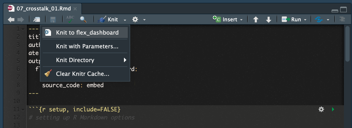
You must click the Knit > Knit to flex_dashboard button to execute and generate the html file.
The repo containing the data and scripts for this section is on Github. To follow along, simply run the lines of code below in R.
We’re going to build this in R Markdown.
The progression of code will be in 07_crosstalk_01.Rmd through 07_crosstalk_04.Rmd.
The data
We’re working with data I’ve already joined and summarized based on raw arcos data.
If you want to see the code looks like, it’s in the script folder called 99_state_pharm_data.R
This is what the summarized data looks like:
library(tidyverse)── Attaching core tidyverse packages ──────────────────────── tidyverse 2.0.0 ──
✔ dplyr 1.1.4 ✔ readr 2.1.4
✔ forcats 1.0.0 ✔ stringr 1.5.1
✔ ggplot2 3.4.3 ✔ tibble 3.2.1
✔ lubridate 1.9.3 ✔ tidyr 1.3.1
✔ purrr 1.0.2
── Conflicts ────────────────────────────────────────── tidyverse_conflicts() ──
✖ dplyr::filter() masks stats::filter()
✖ dplyr::lag() masks stats::lag()
ℹ Use the conflicted package (<http://conflicted.r-lib.org/>) to force all conflicts to become errorsstate <- read_csv("data/all_pharmacies_summarized.csv")Rows: 82813 Columns: 17
── Column specification ────────────────────────────────────────────────────────
Delimiter: ","
chr (10): BUYER_DEA_NO, BUYER_STATE, BUYER_COUNTY, countyfips, BUYER_BUS_ACT...
dbl (7): lat, lon, total_dosage_unit, total_records, average_population, pe...
ℹ Use `spec()` to retrieve the full column specification for this data.
ℹ Specify the column types or set `show_col_types = FALSE` to quiet this message.glimpse(state)Rows: 82,813
Columns: 17
$ BUYER_DEA_NO <chr> "BR5156078", "BW4707139", "BN5150141", "FH2332233",…
$ BUYER_STATE <chr> "AL", "AL", "AL", "AL", "AL", "AL", "AL", "AL", "AL…
$ BUYER_COUNTY <chr> "BALDWIN", "BALDWIN", "BALDWIN", "BALDWIN", "BALDWI…
$ lat <dbl> 30.8804, 30.8859, 30.9046, 30.8838, 30.8826, 30.884…
$ lon <dbl> -87.7845, -87.7867, -87.7839, -87.7893, -87.7734, -…
$ total_dosage_unit <dbl> 1901530, 1481300, 1308370, 326720, 231570, 132680, …
$ total_records <dbl> 2056, 6035, 3902, 1400, 936, 289, 35, 11, 1232, 589…
$ countyfips <chr> "01003", "01003", "01003", "01003", "01003", "01003…
$ average_population <dbl> 175270, 175270, 175270, 175270, 175270, 175270, 175…
$ per_person <dbl> 1.5, 1.2, 1.1, 0.3, 0.2, 0.1, 0.0, 0.0, 1.8, 0.8, 3…
$ BUYER_BUS_ACT <chr> "CHAIN PHARMACY", "CHAIN PHARMACY", "RETAIL PHARMAC…
$ BUYER_NAME <chr> "ALABAMA CVS PHARMACY, L.L.C.", "WINN-DIXIE PHARMAC…
$ BUYER_ADDRESS1 <chr> "208 MCMEANS AVE.", "710 MCMEANS AVE", "2012 HAND A…
$ BUYER_CITY <chr> "BAY MINETTE", "BAY MINETTE", "BAY MINETTE", "BAY M…
$ BUYER_ZIP <dbl> 36507, 36507, 36507, 36507, 36507, 36507, 36535, 36…
$ BUYER_ADDL_CO_INFO <chr> "DBA: CVS/PHARMACY # 04938", NA, NA, "DBA BELL'S H…
$ BUYER_ADDRESS2 <chr> NA, NA, NA, NA, NA, NA, NA, "SUITE 101", NA, "69005…It’s every store in the country. It has total pills (oxycodone and hydrocodone) within the time span of our data. And it has per_person which adjusts total for population by county. Most importantly, each pharmacy has latitude and longitude data so we can use to put these locations on a map.
Setting up the flex dashboard structure
This section is in 07_crosstalk_01.Rmd.
The first thing you’ll notice at the top of the .Rmd file is the text between the — signs. This is the yaml part of the file that tells RStudio how to knit the file. Sometimes the output is pdf, sometimes it’s html, sometime it’s simple markdown.
In this instance, we’re exporting this file as a flex dashboard, with a theme of paper (You could come up with your own theme if your organization wants a consistent style).
---
title: "Crosstalk 1"
author: "NICAR 2020"
date: "3/5/2020"
output:
  flexdashboard::flex_dashboard:
    theme: paper
    source_code: embed
---
Okay, that’s basic.
Beneath it are the sections of code that are indicated with a ```{r.

Anything within this chunk will be treating like a specific code.
The “r” in ```{r indicates that R code will be executed.
If you put in ```{python then Python code would be executed in the R markdown.
Anything outside of these ``` will be treated like regular markdown.
Take the time to learn more ways to customize your R Markdown code.
The important thing to understand is this next set of code that sets up the modules you want to show with flex dashboard. Check out their documentation.
Opioids in State {data-icon="ion-stats-bars"}
=====================================

Column {data-width=200}
-------------------------------------

### Filters
This is specific markdown code that flex dashboard recognizes.
It takes data from the yaml section and the text in the code above and sets the header, the column width and what to name that particular section.
We’re only going to print text in each R code chunk to see where things end up.
Click Knit > Knit to flex_dashboard on the 07_crosstalk_01.Rmd file.
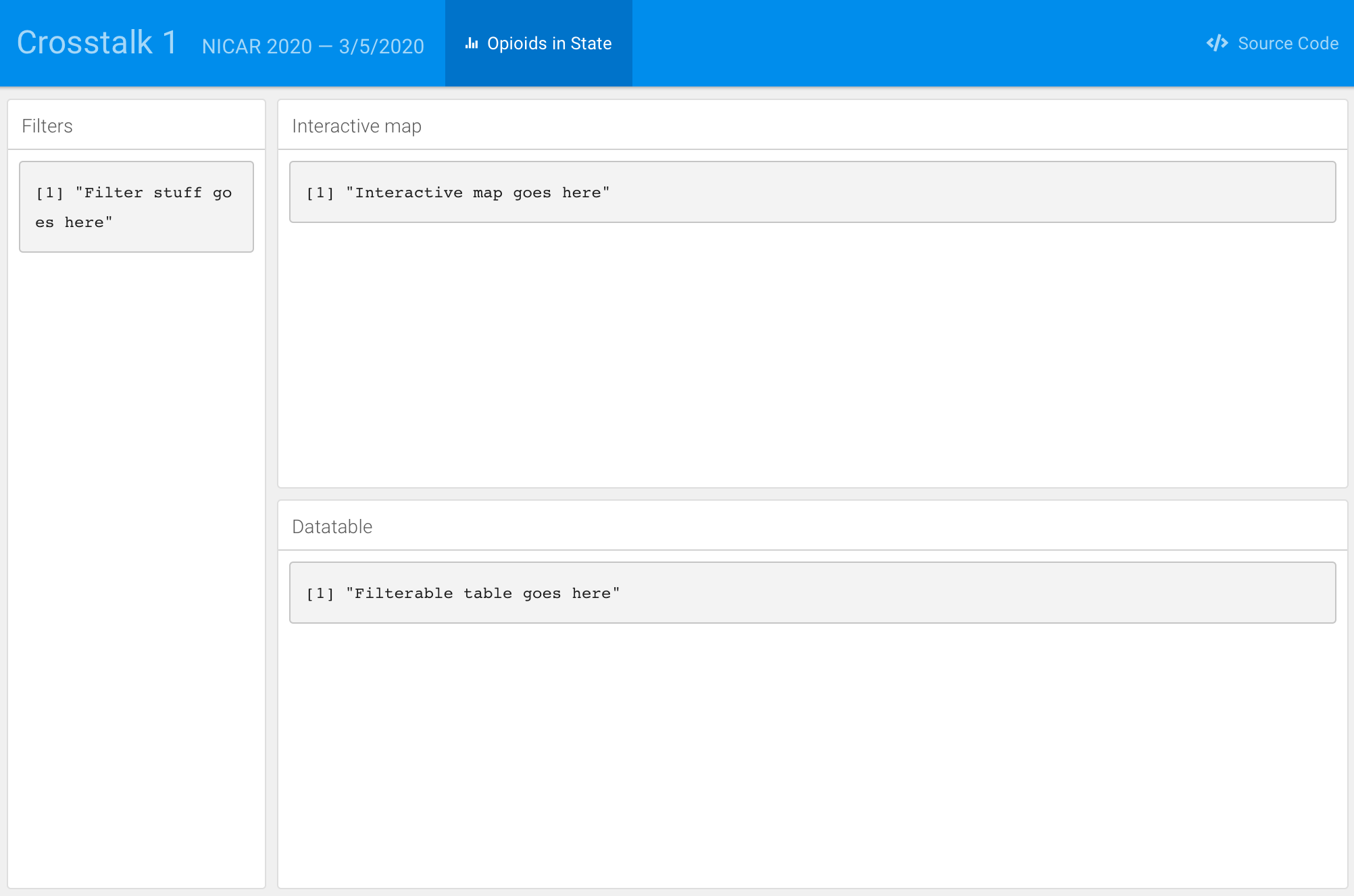
Pretty nice, right?
Even nicer considering how we typed zero HTML and CSS.
Loading and displaying data pt 1
This section is in 07_crosstalk_02.Rmd.
Alright, let’s bring in data and show what it looks like as a filterable table.
We’re going to skip the filtering part for now.
We looked at it in our console already but we need to load it into the R markdown file.
Look in the new chunk called load_and_clean_data

The important takeaway here is that after loading and filtering the data frame and storing it as state, we then used the SharedData$new() function to convert state into a crosstalk object.
This is like an enhanced data set. You’ll see why in a bit.
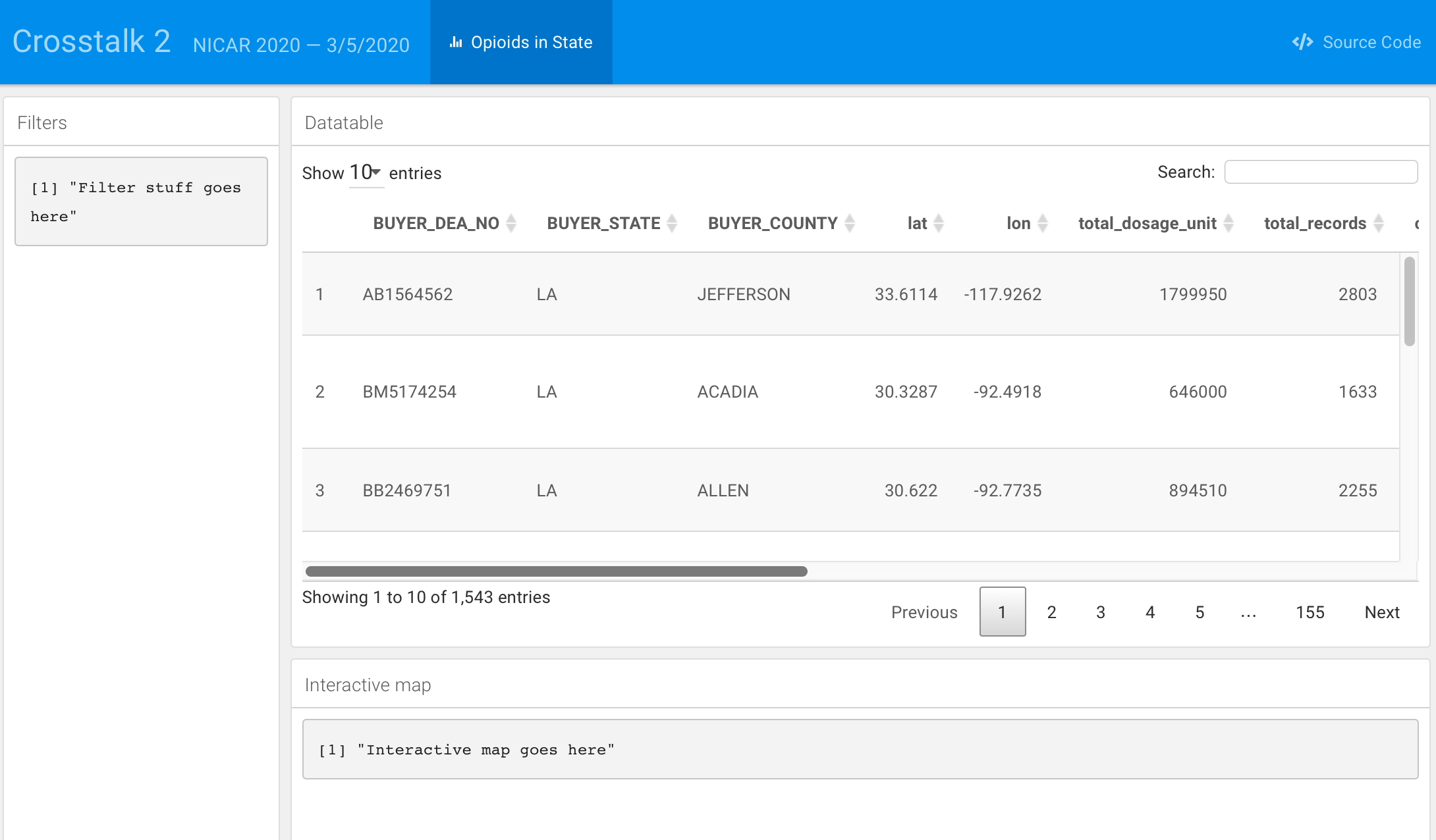
Look at the filterable_table chunk, now.

We’ve used the datatable() function to show the st crosstalk dataframe object.
Click Knit > Knit to flex_dashboard on the 07_crosstalk_02.Rmd file.
Setting up custom filters
This section is in 07_crosstalk_03.Rmd.
We’re going to alter the filter_section code chunk.
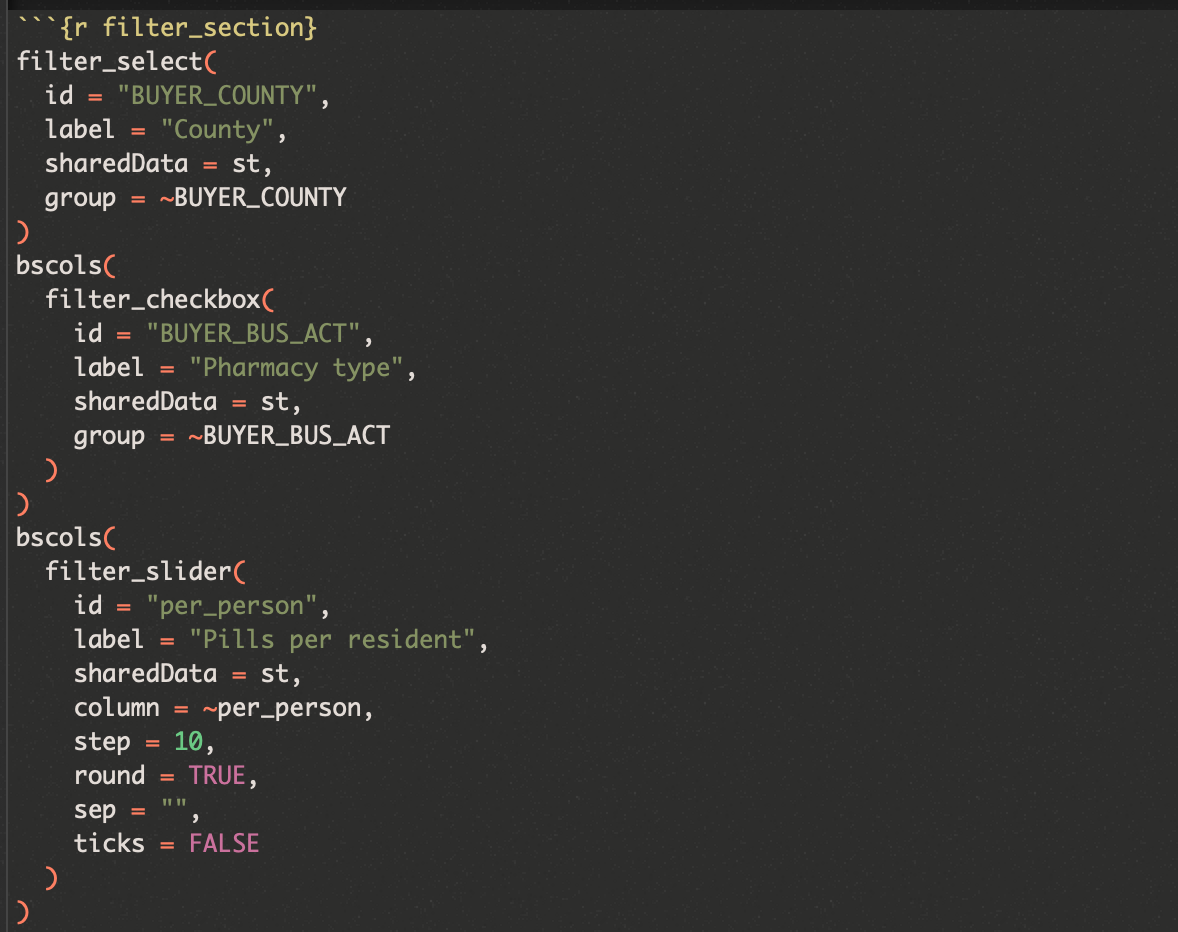
We’re using a few crosstalk specific filter functions: filter_select(), filter_checkbox(), and filter_slider() that will let us choose how to filter the st shared data object.
We’ve wrapped a couple of them around an additional function: bscols() that will pair up a couple of the narrower filters so it looks pretty.
Click Knit > Knit to flex_dashboard on the 07_crosstalk_03.Rmd file.
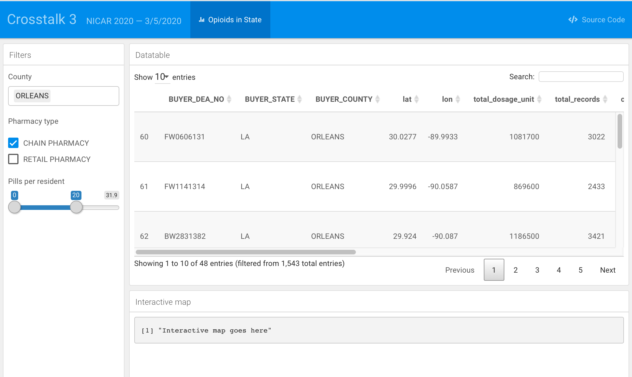
Neat, huh?
When we add filters on the left, either with a pull down menu or with the check box or via the slider bar, the table on the right will automatically update.
Interactive map
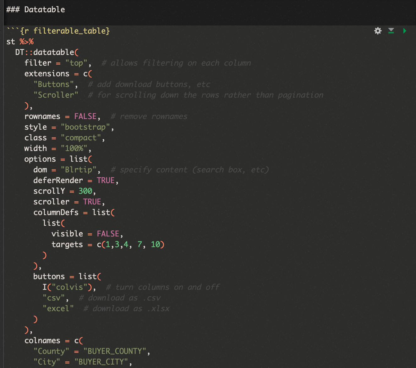
This section is in 07_crosstalk_04.Rmd.
We’re going to alter the interactive_map code chunk.
You’ve gone through the leaflet section before. Now, this is tricky.
We’re starting with the st crosstalk shared object but the values we’re setting for radius (addCircles()) and the text that we’re using to generate the popup text are based on the original state dataframe.
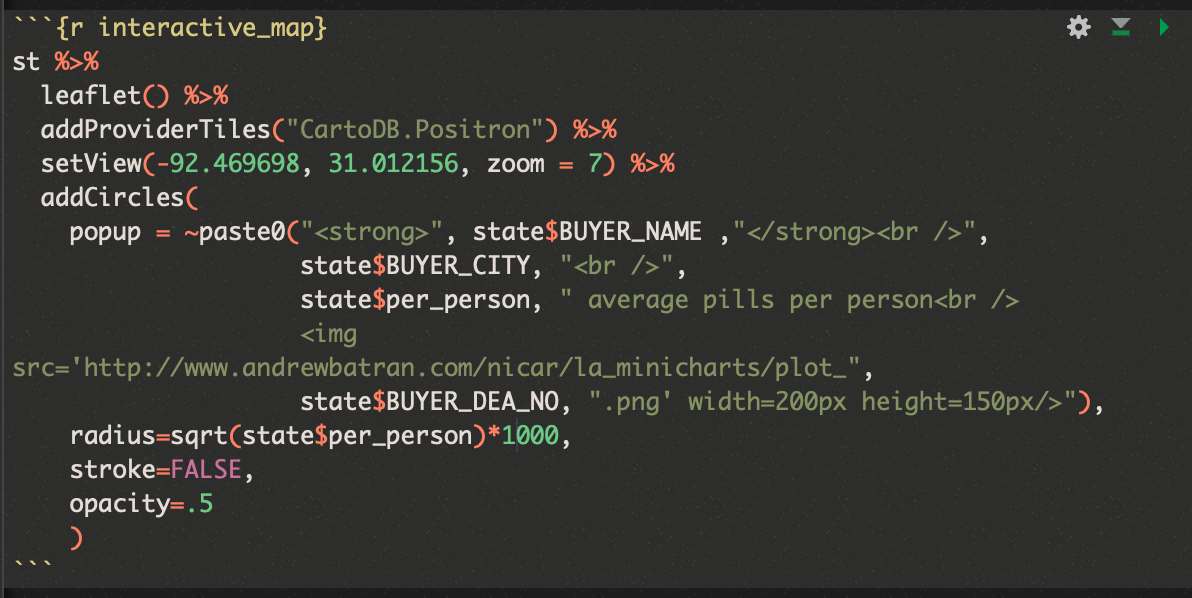
Also, you might have noticed I added some custom images to the popups depending on the BUYER_DEA_NO. These files are specific to Louisiana and show a pharmacy’s monthly opioid ordering trend compared to the state average.
Click Knit > Knit to flex_dashboard on the 07_crosstalk_04.Rmd file.
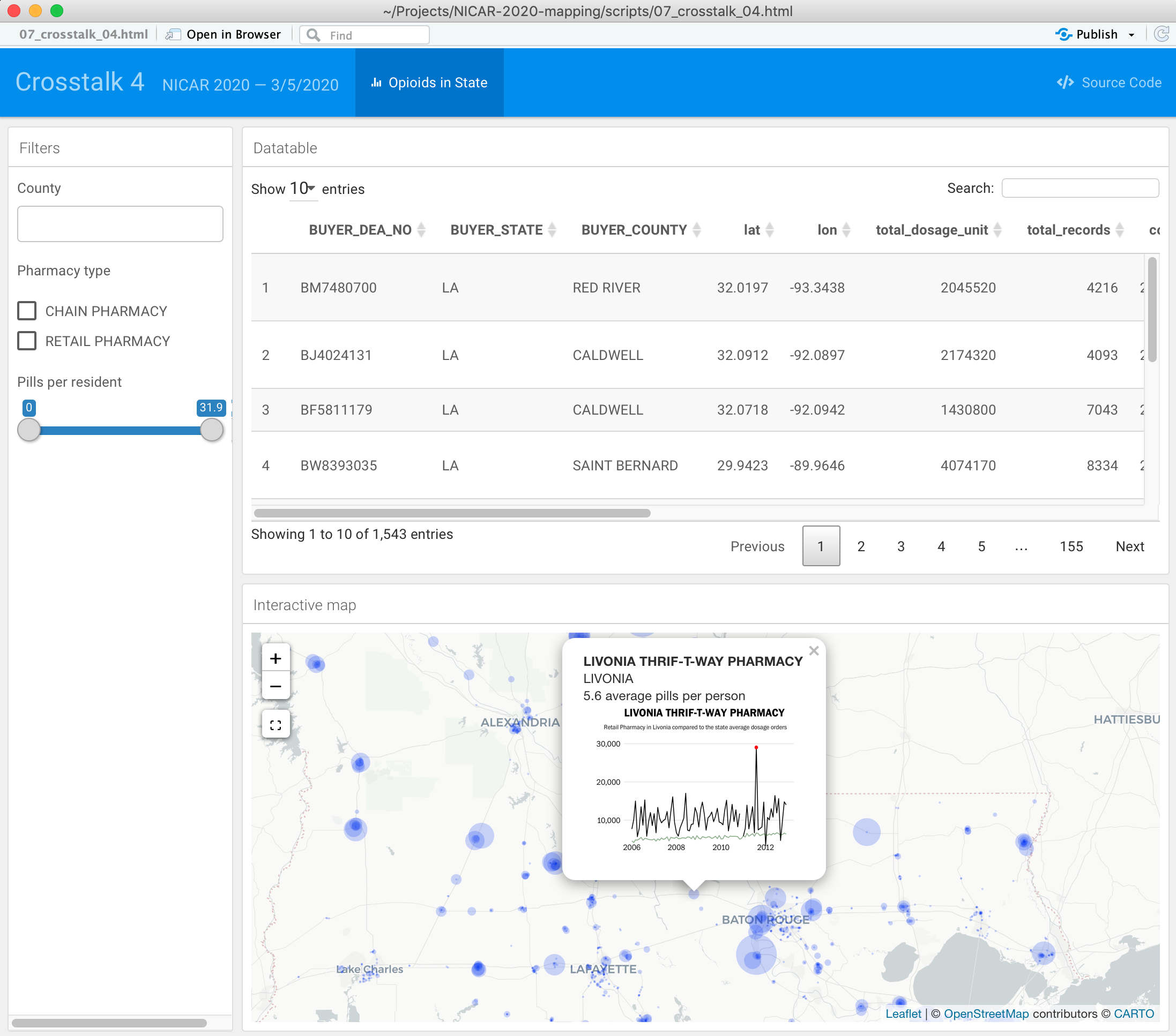
Final datatable options
Almost done. Let’s go back and add some variables to the datable() function so we can add some neat customization to it, such as buttons to export the filtered data and scrolling options.
This section is in 07_crosstalk_05.Rmd.
We’re going to alter the filterable_table code chunk.
Here’s a preview of what we’re changing.
For complete documentation of what’s available as DT options, visit their site.
Click Knit > Knit to flex_dashboard on the 07_crosstalk_05.Rmd file.
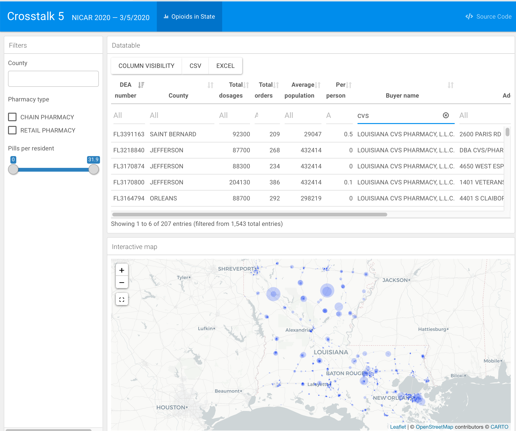
Beautiful, no?