Tidycensus

The repo containing the data and scripts for this section is on Github. To install those files, run the lines of code below.

#install.packages("usethis")
usethis::use_course("https://github.com/r-journalism/nicar-2024-tidycensus/archive/master.zip")

# Run this in the console of RStudio
file.edit("01_tidycensus.R")

# Or click on the 01_tidycensus.R file in the RStudio file explorer tab

To follow along with this walkthrough, simply run the lines of code in the gray boxes in the R console. Be sure to run them in order. If you run into an error, it may be because you skipped running some preceding lines of code.

The American Community Survey from the Census

What is the ACS?

Annual survey of 3.5 million US households
Covers more specific topics not available in decennial US Census data (e.g. income, education, language, housing characteristics)
Available as 1-year estimates (for geographies of population 65,000 and greater) and 5-year estimates (for geographies down to the block group)
Data delivered as estimates characterized by margins of error

How to get ACS data

tidycensus

Load libraries

library(tidyverse)
library(tidycensus)

Census data issues I

Groups, sub groups, sub sub groups, etc, are a pain
Takes forever to tidy up

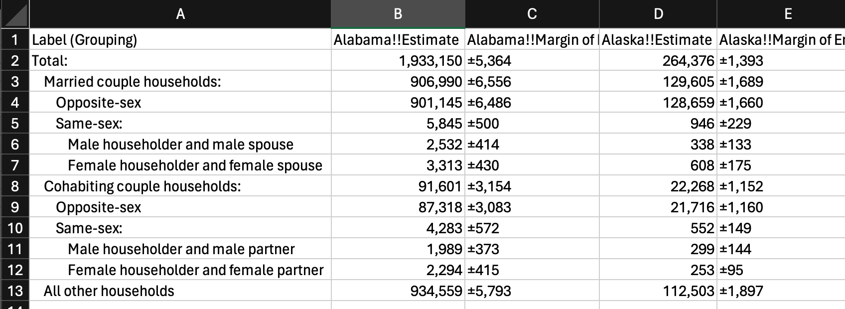
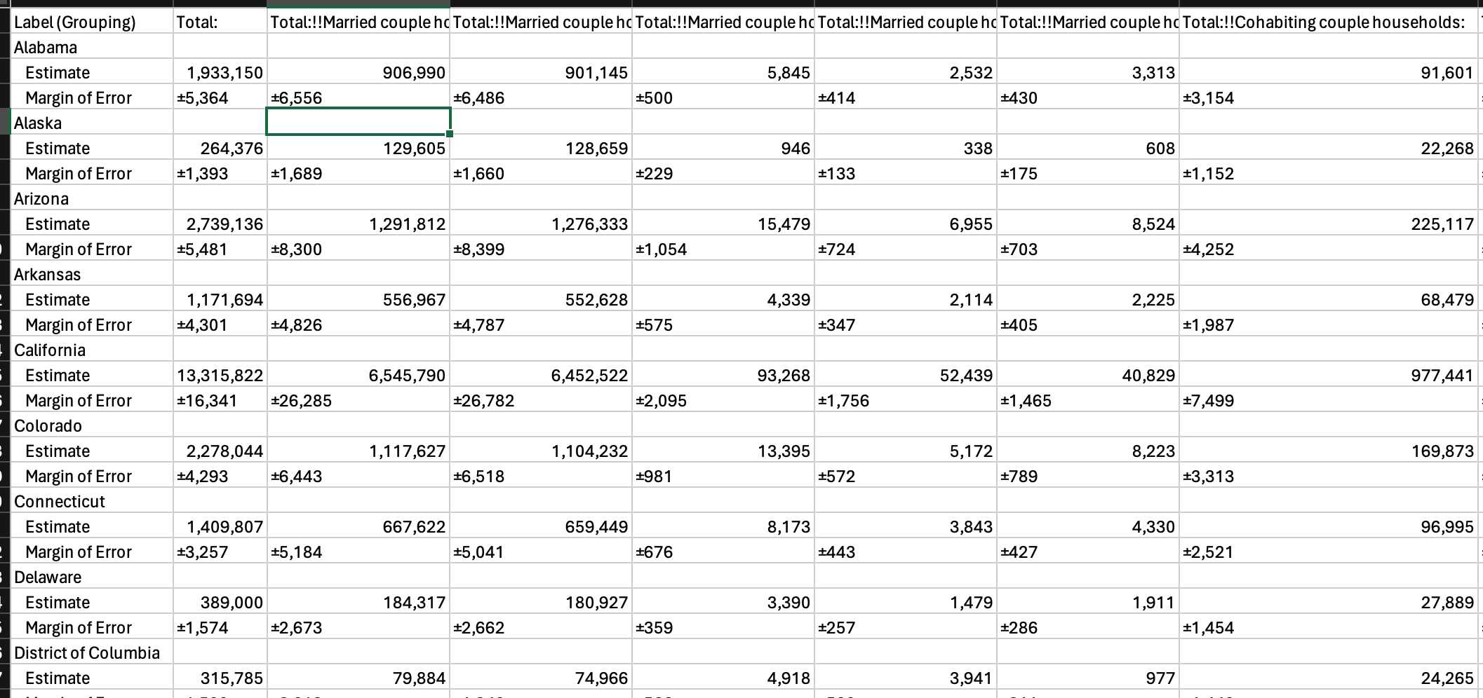
Census data issues II

Transposing the data helps a bit but
Still requires a lot of work to clean up

Tidycensus: Features

Wrangles Census data internally to return tidyverse-ready format (or traditional wide format if requested)
Automatically downloads and merges Census geometries to data for mapping
Includes tools for handling margins of error in the ACS and working with survey weights in the ACS PUMS
States and counties can be requested by name (no more looking up FIPS codes!)
Script out your process for re usability

R and RStudio

R: programming language and software environment for data analysis (and scraping and visualization and so much more)
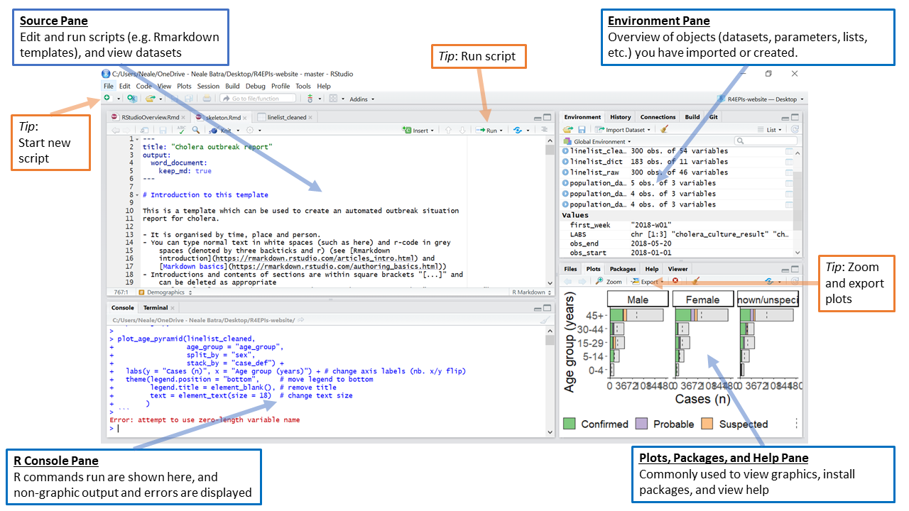
RStudio: integrated development environment (IDE) for R developed by Posit
- Built on top of R
- Lets you view your data, write and save R (or Python) scripts or notebooks, and view graphical static and interactive outputs

RStudio tour

Running code in R

<- assignment saves to the environment/memory
# hashes, commented out code
- Copy and paste code into the console to run (without the hash)
run code in the console at the bottom or
in a script, highlight the code and click the ‘run’ button at the top right
or put your cursor in the script on the line of code and hit ctrl+enter (or cmd + enter)

Getting started with tidycensus

To get started, install the packages and files for this class
If you are using an IRE laptop, these packages are already installed for you

install.packages(c("tidycensus", "tidyverse", "mapview", "usethis"))
usethis::use_course("https://github.com/r-journalism/nicar-2024-tidycensus/archive/master.zip")

Optional: your Census API key

tidycensus (and the Census API) can be used without an API key, but you will be limited to 500 queries per day
Power users: visit https://api.census.gov/data/key_signup.html to request a key, then activate the key from the link in your email.
Once activated, use the census_api_key() function to set your key as an environment variable

library(tidycensus)

census_api_key("YOUR KEY GOES HERE", install = TRUE)

Getting started with ACS data in tidycensus

open 01_tidycensus.R in RStudio

Using the `get_acs()` function

The get_acs() function is your portal to access ACS data using tidycensus
The two required arguments are geography and variables. The function defaults to the latest 5-year ACS (Currently 2018-2022)

library(tidycensus)

median_income <- get_acs(
  geography = "county",
  variables = "B25077_001", # median household income
  year = 2022
)

Getting data from the 2018-2022 5-year ACS

ACS data are returned with five columns: GEOID, NAME, variable, estimate, and moe

median_income

# A tibble: 3,222 × 5
   GEOID NAME                     variable   estimate   moe
   <chr> <chr>                    <chr>         <dbl> <dbl>
 1 01001 Autauga County, Alabama  B25077_001   191800  7996
 2 01003 Baldwin County, Alabama  B25077_001   266000  6916
 3 01005 Barbour County, Alabama  B25077_001   102700 11171
 4 01007 Bibb County, Alabama     B25077_001   120100 13377
 5 01009 Blount County, Alabama   B25077_001   159800  6189
 6 01011 Bullock County, Alabama  B25077_001    87700 20560
 7 01013 Butler County, Alabama   B25077_001    94800  5984
 8 01015 Calhoun County, Alabama  B25077_001   140500  5181
 9 01017 Chambers County, Alabama B25077_001   116900  9814
10 01019 Cherokee County, Alabama B25077_001   158700  8550
# ℹ 3,212 more rows

Exploring your data with RStudio

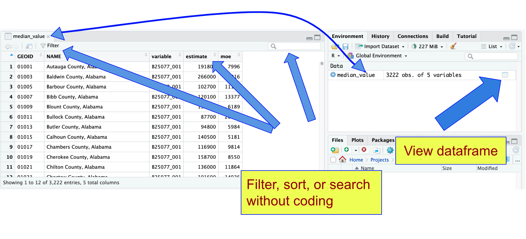
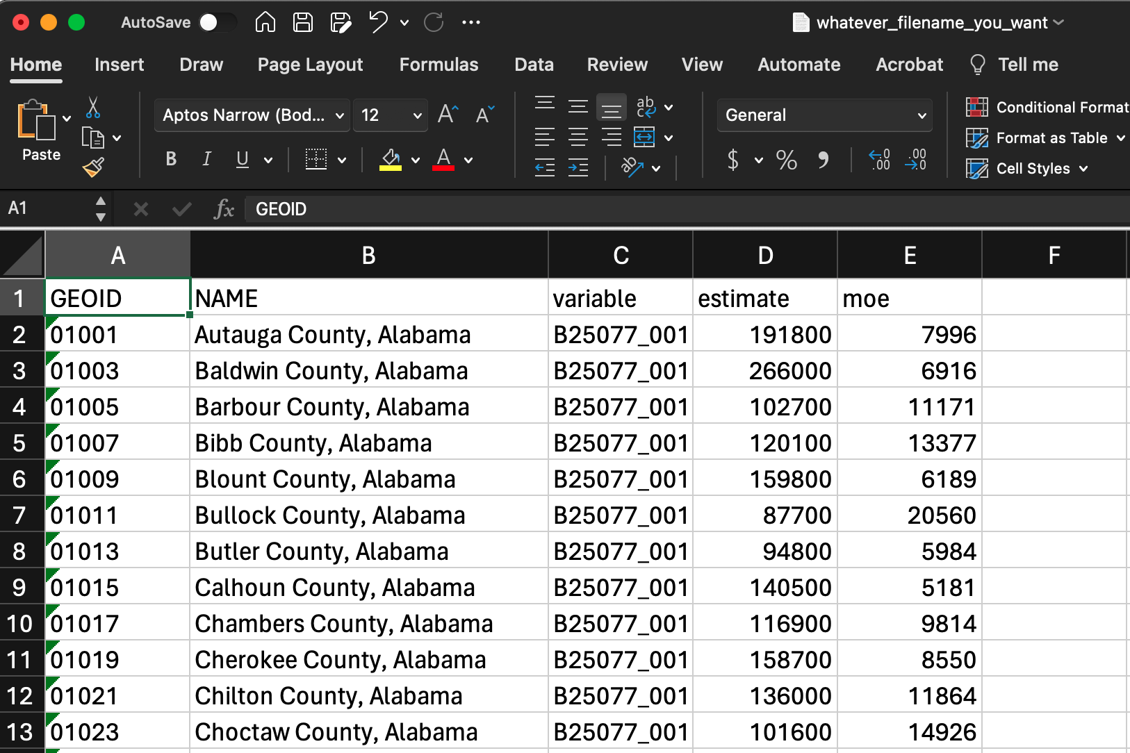
View(median_income)

Exporting your data

You saved the output of the get_acs() function to the object median_income
Export that dataframe object to your computer so you can use it wherever you want

library(readr)

write_csv(median_income, "whatever_filename_you_want.csv", na="")

Take your data to Excel if you want

1-year ACS data

1-year ACS data are more current, but are only available for geographies of population 65,000 and greater
Access 1-year ACS data with the argument survey = "acs1"; defaults to "acs5"

median_value_1yr <- get_acs(
  geography = "place",
  variables = "B25077_001", # median value of homes
  year = 2022,
  survey = "acs1"
)

Getting data from the 2022 1-year ACS

The 1-year ACS provides data for geographies with populations of 65,000 and greater.

median_value_1yr

# A tibble: 646 × 5
   GEOID   NAME                           variable   estimate   moe
   <chr>   <chr>                          <chr>         <dbl> <dbl>
 1 0103076 Auburn city, Alabama           B25077_001   335200 22622
 2 0107000 Birmingham city, Alabama       B25077_001   125500 14964
 3 0121184 Dothan city, Alabama           B25077_001   190800  8133
 4 0135896 Hoover city, Alabama           B25077_001   393400 19743
 5 0137000 Huntsville city, Alabama       B25077_001   294700 16881
 6 0150000 Mobile city, Alabama           B25077_001   178800 11552
 7 0151000 Montgomery city, Alabama       B25077_001   155200 10868
 8 0177256 Tuscaloosa city, Alabama       B25077_001   297600 30475
 9 0203000 Anchorage municipality, Alaska B25077_001   367900 10111
10 0404720 Avondale city, Arizona         B25077_001   400300 22495
# ℹ 636 more rows

Requesting tables of variables

The table parameter can be used to obtain all related variables in a “table” at once

income_table <- get_acs(
  geography = "county", 
  table = "B19001", 
  year = 2022
)

Getting data from the 2018-2022 5-year ACS

Loading ACS5 variables for 2022 from table B19001. To cache this dataset for faster access to ACS tables in the future, run this function with `cache_table = TRUE`. You only need to do this once per ACS dataset.

income_table

# A tibble: 54,774 × 5
   GEOID NAME                    variable   estimate   moe
   <chr> <chr>                   <chr>         <dbl> <dbl>
 1 01001 Autauga County, Alabama B19001_001    22308   369
 2 01001 Autauga County, Alabama B19001_002      990   265
 3 01001 Autauga County, Alabama B19001_003      656   187
 4 01001 Autauga County, Alabama B19001_004     1026   303
 5 01001 Autauga County, Alabama B19001_005     1335   329
 6 01001 Autauga County, Alabama B19001_006      741   205
 7 01001 Autauga County, Alabama B19001_007      822   218
 8 01001 Autauga County, Alabama B19001_008      840   270
 9 01001 Autauga County, Alabama B19001_009      921   260
10 01001 Autauga County, Alabama B19001_010      962   279
# ℹ 54,764 more rows

Understanding geography and variables in tidycensus

US Census Geography

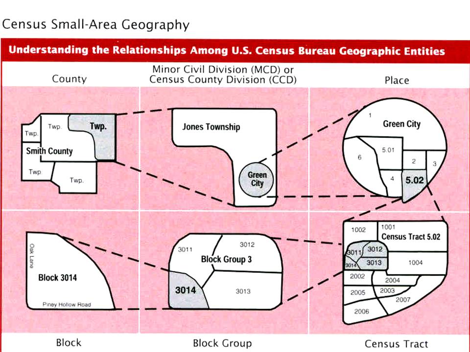
Geography in tidycensus

Information on available geographies, and how to specify them, can be found in the tidycensus documentation

Geography	Definition	Available by	Available in
`"us"`	United States		`get_acs()`, `get_decennial()`
`"region"`	Census region		`get_acs()`, `get_decennial()`
`"division"`	Census division		`get_acs()`, `get_decennial()`
`"state"`	State or equivalent	state	`get_acs()`, `get_decennial()`
`"county"`	County or equivalent	state, county	`get_acs()`, `get_decennial()`
`"county subdivision"`	County subdivision	state, county	`get_acs()`, `get_decennial()`
`"tract"`	Census tract	state, county	`get_acs()`, `get_decennial()`
`"block group"` OR `"cbg"`	Census block group	state, county	`get_acs()`, `get_decennial()`

Querying by state

For geographies available below the state level, the state parameter allows you to query data for a specific state
For smaller geographies (Census tracts, block groups), a county argument may also need to be included
tidycensus translates state names and postal abbreviations internally, so you don’t need to remember the FIPS codes!

Querying tract data requires county and state

Example: data on median home value in San Diego County, California by Census tract

sd_value <- get_acs(
  geography = "tract", 
  variables = "B25077_001", 
  state = "CA", 
  county = "San Diego",
  year = 2022
)

Getting data from the 2018-2022 5-year ACS

sd_value

# A tibble: 737 × 5
   GEOID       NAME                                     variable estimate    moe
   <chr>       <chr>                                    <chr>       <dbl>  <dbl>
 1 06073000100 Census Tract 1; San Diego County; Calif… B25077_…  1633800  71171
 2 06073000201 Census Tract 2.01; San Diego County; Ca… B25077_…  1331000 147432
 3 06073000202 Census Tract 2.02; San Diego County; Ca… B25077_…   891100  97240
 4 06073000301 Census Tract 3.01; San Diego County; Ca… B25077_…   957500 232555
 5 06073000302 Census Tract 3.02; San Diego County; Ca… B25077_…   761700 108681
 6 06073000400 Census Tract 4; San Diego County; Calif… B25077_…   799100  94490
 7 06073000500 Census Tract 5; San Diego County; Calif… B25077_…  1025000  81768
 8 06073000600 Census Tract 6; San Diego County; Calif… B25077_…   727700  92078
 9 06073000700 Census Tract 7; San Diego County; Calif… B25077_…   736400 102788
10 06073000800 Census Tract 8; San Diego County; Calif… B25077_…   678400 119751
# ℹ 727 more rows

Searching for variables

To search for variables, use the load_variables() function along with a year and dataset
The View() function in RStudio allows for interactive browsing and filtering

vars <- load_variables(2022, "acs5")

View(vars)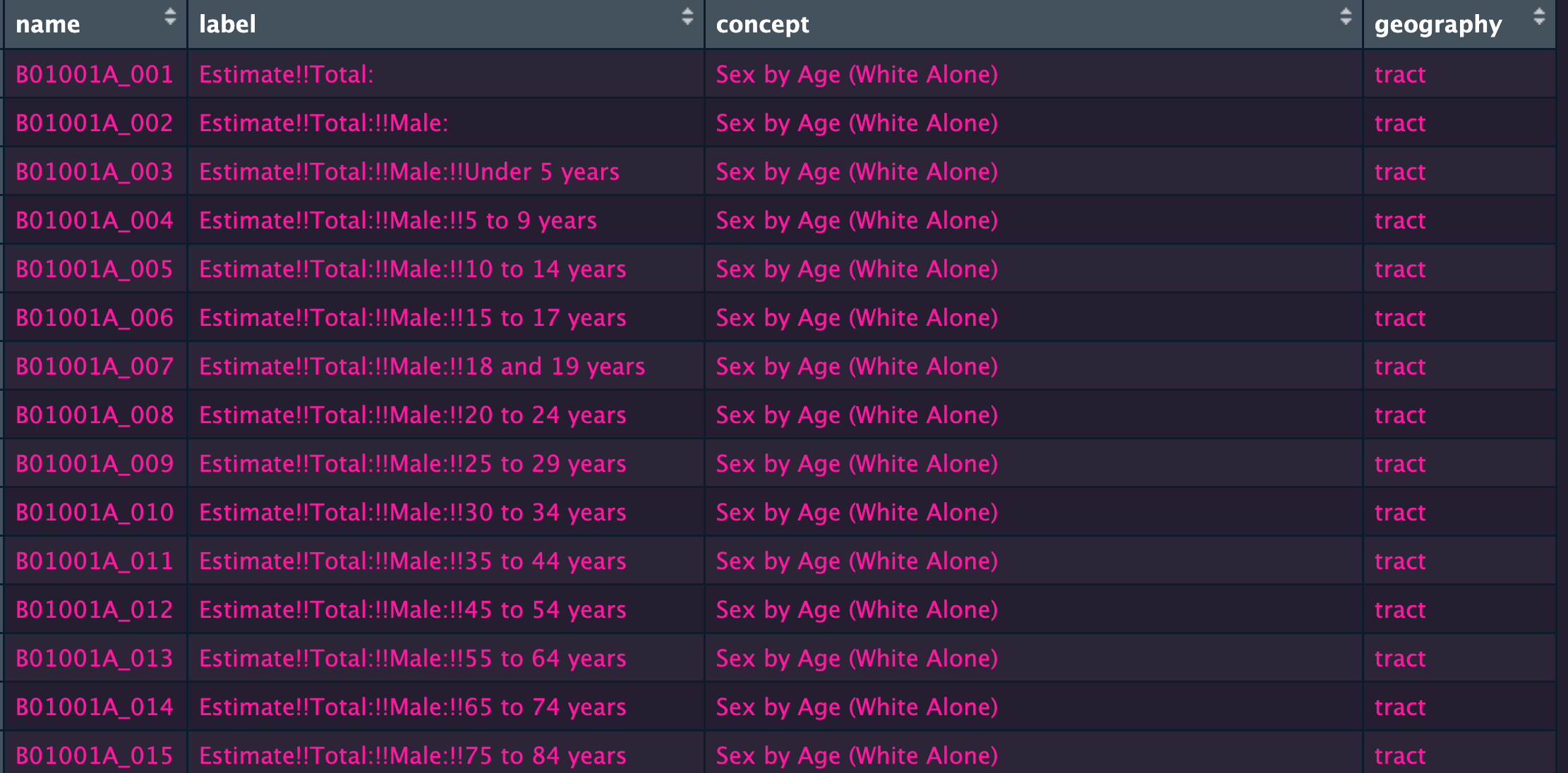

Available ACS datasets in tidycensus

Detailed Tables
Data Profile (add "/profile" for variable lookup)
Subject Tables (add "/subject")
Comparison Profile (add "/cprofile")
Supplemental Estimates (use "acsse")
Migration Flows (access with get_flows())

Data structure in tidycensus

“Tidy” or long-form data

The default data structure returned by tidycensus is “tidy” or long-form data, with variables by geography stacked by row

age_sex_table <- get_acs(
  geography = "state", 
  table = "B01001", 
  year = 2022,
  survey = "acs1",
)

Getting data from the 2022 1-year ACS

The 1-year ACS provides data for geographies with populations of 65,000 and greater.

Loading ACS1 variables for 2022 from table B01001. To cache this dataset for faster access to ACS tables in the future, run this function with `cache_table = TRUE`. You only need to do this once per ACS dataset.

age_sex_table

# A tibble: 2,548 × 5
   GEOID NAME    variable   estimate   moe
   <chr> <chr>   <chr>         <dbl> <dbl>
 1 01    Alabama B01001_001  5074296    NA
 2 01    Alabama B01001_002  2461248  6178
 3 01    Alabama B01001_003   146169  3134
 4 01    Alabama B01001_004   158767  6029
 5 01    Alabama B01001_005   164578  5689
 6 01    Alabama B01001_006    97834  3029
 7 01    Alabama B01001_007    70450  2897
 8 01    Alabama B01001_008    42597  4156
 9 01    Alabama B01001_009    34623  3440
10 01    Alabama B01001_010    97373  4627
# ℹ 2,538 more rows

“Wide” data

The argument output = "wide" spreads Census variables across the columns, returning one row per geographic unit and one column per variable

age_sex_table_wide <- get_acs(
  geography = "state", 
  table = "B01001", 
  year = 2022,
  survey = "acs1",
  output = "wide" 
)

Getting data from the 2022 1-year ACS

The 1-year ACS provides data for geographies with populations of 65,000 and greater.

Loading ACS1 variables for 2022 from table B01001. To cache this dataset for faster access to ACS tables in the future, run this function with `cache_table = TRUE`. You only need to do this once per ACS dataset.

age_sex_table_wide

# A tibble: 52 × 100
   GEOID NAME        B01001_001E B01001_001M B01001_002E B01001_002M B01001_003E
   <chr> <chr>             <dbl>       <dbl>       <dbl>       <dbl>       <dbl>
 1 01    Alabama         5074296          NA     2461248        6178      146169
 2 02    Alaska           733583          NA      385667        2351       23043
 3 04    Arizona         7359197          NA     3678381        2695      201423
 4 05    Arkansas        3045637          NA     1504488        4216       90239
 5 06    California     39029342          NA    19536425        6410     1081904
 6 08    Colorado        5839926          NA     2960896        4278      154565
 7 09    Connecticut     3626205          NA     1776689        2237       91513
 8 10    Delaware        1018396          NA      494657        1092       27456
 9 11    District o…      671803          NA      319763         733       20038
10 12    Florida        22244823          NA    10953468        6169      563703
# ℹ 42 more rows
# ℹ 93 more variables: B01001_003M <dbl>, B01001_004E <dbl>, B01001_004M <dbl>,
#   B01001_005E <dbl>, B01001_005M <dbl>, B01001_006E <dbl>, B01001_006M <dbl>,
#   B01001_007E <dbl>, B01001_007M <dbl>, B01001_008E <dbl>, B01001_008M <dbl>,
#   B01001_009E <dbl>, B01001_009M <dbl>, B01001_010E <dbl>, B01001_010M <dbl>,
#   B01001_011E <dbl>, B01001_011M <dbl>, B01001_012E <dbl>, B01001_012M <dbl>,
#   B01001_013E <dbl>, B01001_013M <dbl>, B01001_014E <dbl>, …

Using named vectors of variables

Census variables can be hard to remember; using a named vector to request variables will replace the Census IDs with a custom input
In long form, these custom inputs will populate the variable column; in wide form, they will replace the column names

Renaming variables easily

ca_education <- get_acs(
  geography = "county",
  state = "CA",
  variables = c(percent_high_school = "DP02_0062P", 
                percent_bachelors = "DP02_0065P",
                percent_graduate = "DP02_0066P"), 
  year = 2021
)

Getting data from the 2017-2021 5-year ACS

Using the ACS Data Profile

ca_education

# A tibble: 174 × 5
   GEOID NAME                       variable            estimate   moe
   <chr> <chr>                      <chr>                  <dbl> <dbl>
 1 06001 Alameda County, California percent_high_school     16.7   0.4
 2 06001 Alameda County, California percent_bachelors       28.3   0.3
 3 06001 Alameda County, California percent_graduate        21.3   0.3
 4 06003 Alpine County, California  percent_high_school     25.7   7.5
 5 06003 Alpine County, California  percent_bachelors       20.6   7.5
 6 06003 Alpine County, California  percent_graduate        18.7   8.5
 7 06005 Amador County, California  percent_high_school     30.7   2.2
 8 06005 Amador County, California  percent_bachelors       13.6   1.8
 9 06005 Amador County, California  percent_graduate         5.9   1.1
10 06007 Butte County, California   percent_high_school     22.3   0.9
# ℹ 164 more rows

ACS data warnings

Understanding limitations of the 1-year ACS

The 1-year American Community Survey is only available for geographies with population 65,000 and greater. This means:
Only 848 of 3,221 counties are available
Only 646 of 31,908 cities / Census-designated places are available
No data for Census tracts, block groups, ZCTAs, or any other geographies that typically have populations below 65,000

Data sparsity and margins of error

You may encounter data issues in the 1-year ACS data that are less pronounced in the 5-year ACS. For example:
Values available in the 5-year ACS may not be available in the corresponding 1-year ACS tables
If available, they will likely have larger margins of error
Your job as an data journalist: balance need for certainty vs. need for recency in estimates

Tagalog speakers by state (1-year ACS)

get_acs(
  geography = "state",
  variables = "B16001_099",
  year = 2022,
  survey = "acs1"
)

Getting data from the 2022 1-year ACS

The 1-year ACS provides data for geographies with populations of 65,000 and greater.

# A tibble: 52 × 5
   GEOID NAME                 variable   estimate   moe
   <chr> <chr>                <chr>         <dbl> <dbl>
 1 01    Alabama              B16001_099     5222  1487
 2 02    Alaska               B16001_099       NA    NA
 3 04    Arizona              B16001_099    28522  3746
 4 05    Arkansas             B16001_099       NA    NA
 5 06    California           B16001_099   760215 22953
 6 08    Colorado             B16001_099     9417  2178
 7 09    Connecticut          B16001_099     8568  2657
 8 10    Delaware             B16001_099     1112   601
 9 11    District of Columbia B16001_099       NA    NA
10 12    Florida              B16001_099    80209  7025
# ℹ 42 more rows

Tagalog speakers by state (5-year ACS)

get_acs(
  geography = "state",
  variables = "B16001_099",
  year = 2022,
  survey = "acs5"
)

Getting data from the 2018-2022 5-year ACS

# A tibble: 52 × 5
   GEOID NAME                 variable   estimate   moe
   <chr> <chr>                <chr>         <dbl> <dbl>
 1 01    Alabama              B16001_099     3854   553
 2 02    Alaska               B16001_099    18520  1414
 3 04    Arizona              B16001_099    25913  1774
 4 05    Arkansas             B16001_099     3154   515
 5 06    California           B16001_099   772833 10558
 6 08    Colorado             B16001_099     8724   834
 7 09    Connecticut          B16001_099     8353   969
 8 10    Delaware             B16001_099     2837   668
 9 11    District of Columbia B16001_099     1250   306
10 12    Florida              B16001_099    70430  2877
# ℹ 42 more rows

Other warnings

Variables in the Data Profile and Subject Tables can change names over time
The 2022 ACS is the first to include the new Connecticut Planning Regions in the “county” geography

The 2020 Decennial US Census data and R

What is the decennial US Census?

Complete count of the US population mandated by Article 1, Sections 2 and 9 in the US Constitution
Directed by the US Census Bureau (US Department of Commerce); conducted every 10 years since 1790
Used for proportional representation / congressional redistricting
Limited set of questions asked about race, ethnicity, age, sex, and housing tenure

2020 US Census datasets

The PL 94-171 Redistricting Data
The Demographic and Housing Characteristics (DHC) file
The Demographic Profile (for pre-tabulated variables)
Tabulations for the 118th Congress & for Island Areas
The Detailed DHC-A file (with very detailed racial & ethnic categories)

2020 US Census in Tidycensus

The get_decennial() function is used to acquire data from the decennial US Census
The two required arguments are geography and variables for the functions to work; for 2020 Census data, use year = 2020.

pop20 <- get_decennial(
  geography = "state",
  variables = "P1_001N",
  year = 2020
)

Getting data from the 2020 decennial Census

Using the PL 94-171 Redistricting Data Summary File

Note: 2020 decennial Census data use differential privacy, a technique that
introduces errors into data to preserve respondent confidentiality.
ℹ Small counts should be interpreted with caution.
ℹ See https://www.census.gov/library/fact-sheets/2021/protecting-the-confidentiality-of-the-2020-census-redistricting-data.html for additional guidance.
This message is displayed once per session.

Decennial Census data are returned with four columns: GEOID, NAME, variable, and value

pop20

# A tibble: 52 × 4
   GEOID NAME                 variable    value
   <chr> <chr>                <chr>       <dbl>
 1 42    Pennsylvania         P1_001N  13002700
 2 06    California           P1_001N  39538223
 3 54    West Virginia        P1_001N   1793716
 4 49    Utah                 P1_001N   3271616
 5 36    New York             P1_001N  20201249
 6 11    District of Columbia P1_001N    689545
 7 02    Alaska               P1_001N    733391
 8 12    Florida              P1_001N  21538187
 9 45    South Carolina       P1_001N   5118425
10 38    North Dakota         P1_001N    779094
# ℹ 42 more rows

Scavenger hunt

Can you look through the vars table you loaded earlier and import the table that can answer this?

How many 18 to 24 year old Korean people are there in the US (2021)?
What percent of females in 2017 were below poverty level in the US (5 year)?

vars <- load_variables(2022, "acs5")

get_acs(replace_this_with_the_right_arguments)

_How do you find the “right” variables or Census table ID? I do a couple things: Use CensusReporter.org or I ask the oldest data reporter in the newsroom.